
**I. Overview of the Least Mean Square Algorithm (LMS)**
In 1959, Widrow and Hoff introduced the Least Mean Square (LMS) algorithm while researching adaptive linear elements for pattern recognition. The LMS algorithm is based on Wiener filtering but improves upon it by using the steepest descent method. While the Wiener solution requires prior statistical knowledge of the input and desired signals, including the autocorrelation matrix, it is only theoretically optimal. To overcome this limitation, the LMS algorithm approximates the Wiener solution in a recursive way, eliminating the need for matrix inversion. Instead of using the mean square error, it uses the instantaneous error squared, leading to a computationally efficient approach.
Due to its low computational complexity, good convergence properties in stationary environments, unbiased convergence toward the Wiener solution, and stability under limited precision, the LMS algorithm has become one of the most widely used adaptive algorithms. It is known for its simplicity and effectiveness in real-time applications.
The following figure illustrates the vector signal flow of the LMS algorithm:
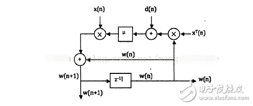
Figure 1: LMS Algorithm Vector Signal Flow Chart
As shown in Figure 1, the LMS algorithm involves two main stages: filtering and adaptation. The general steps of the algorithm are as follows: 1. **Determine parameters**: Set the global step size parameter β and the number of filter taps (also known as the filter order). 2. **Initialize the filter weights**: Choose an initial value for the weight vector. 3. **Algorithm operation**: - Filtered output: $ y(n) = w^T(n)x(n) $ - Error signal: $ e(n) = d(n) - y(n) $ - Weight update: $ w(n+1) = w(n) + \beta e(n)x(n) $ **II. Performance Analysis** The choice of an adaptive algorithm significantly influences the performance of an adaptive filter. Therefore, analyzing the performance of the most commonly used algorithms is crucial. In a stationary environment, key performance metrics include convergence, convergence speed, steady-state error, and computational complexity. 1. **Convergence** Convergence refers to the process where the filter weight vector approaches the optimal value as the number of iterations increases. A well-designed algorithm ensures that the weights eventually stabilize near the optimal solution. 2. **Convergence Speed** This measures how quickly the filter weight vector moves from its initial value to the optimal solution. Faster convergence is generally desirable, especially in real-time applications. 3. **Steady-State Error** Once the algorithm reaches a steady state, the steady-state error represents the deviation between the current weights and the optimal solution. Lower steady-state error indicates better performance. 4. **Computational Complexity** This refers to the amount of computation required to update the filter weights. The LMS algorithm is known for its low computational complexity, making it suitable for resource-constrained systems. **III. Classification of the LMS Algorithm** There are several variations of the LMS algorithm designed to address specific challenges and improve performance under different conditions. 1. **Quantization Error LMS Algorithm** In high-speed applications like echo cancellation or channel equalization, reducing computational load is critical. The quantization error LMS algorithm minimizes computations by quantizing the error signal, such as in symbolic error or symbol data LMS methods. 2. **De-correlated LMS Algorithm** The basic LMS assumes that input signals are statistically independent. When this assumption is violated, the algorithm's performance degrades, particularly in terms of convergence speed. De-correlation techniques, such as time-domain or transform-domain approaches, can enhance convergence. 3. **Parallel Delay LMS Algorithm** This variant is designed for VLSI implementation, leveraging parallelism and pipelining. However, when the filter order is long, the delay introduced can negatively impact convergence performance. 4. **Adaptive Lattice LMS Algorithm** Unlike traditional LMS filters, which assume a fixed order, the lattice-based approach allows for dynamic adjustment of the filter order. This makes it more flexible and efficient in scenarios where the optimal order is unknown. 5. **Newton-LMS Algorithm** This algorithm estimates second-order statistics of the input signal to accelerate convergence, especially when the input is highly correlated. However, it involves computing the inverse of the correlation matrix, which can be computationally intensive and numerically unstable.
The material of this product is PC+ABS. All condition of our product is 100% brand new. OEM and ODM are avaliable of our products for your need. We also can produce the goods according to your specific requirement.
Our products built with input/output overvoltage protection, input/output overcurrent protection, over temperature protection, over power protection and short circuit protection. You can send more details of this product, so that we can offer best service to you!
Led Adapter,Mini Led Adapter,Security Led Adapter,Waterproof Led Adapter
Shenzhen Waweis Technology Co., Ltd. , https://www.waweis.com